RESEARCH NOTE / November 7, 2026
DR-SAC: Robust to the Worst Plausible World, Cheaply
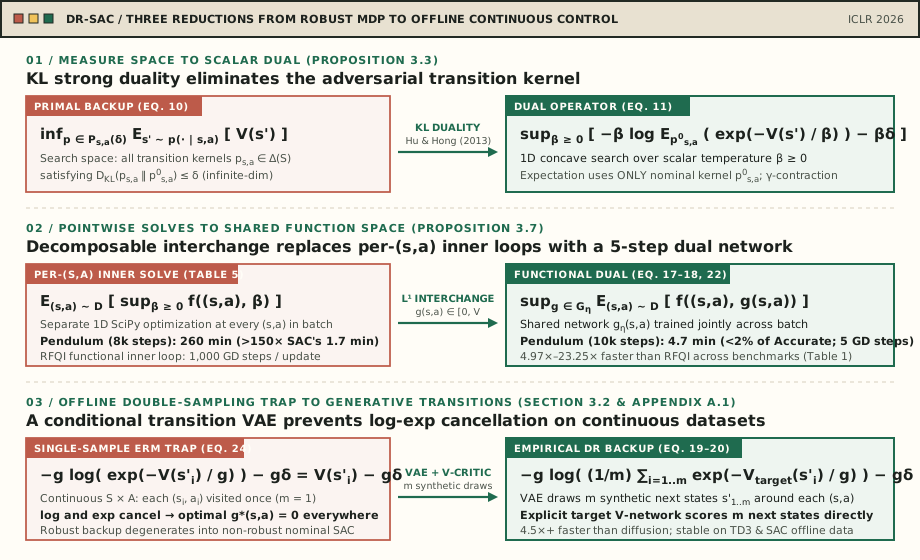
The bottleneck in distributionally robust RL is not defining the worst-case transition model, but making the worst-case soft Bellman backup computable: KL duality, decomposable functional optimization, and a conditional transition VAE turn an infinite-dimensional measure problem into a five-step update inside Soft Actor-Critic.
DR-SAC: Distributionally Robust Soft Actor-Critic for Reinforcement Learning under Uncertainty · ICLR 2026
Mingxuan Cui*, Duo Zhou*†, Yuxuan Han, Grani A. Hanasusanto, Qiong Wang, Huan Zhang, Zhengyuan Zhou
OpenReview · arXiv · PDF · Code · Project page
In distributionally robust reinforcement learning (DR-RL), writing down the worst-case objective is straightforward: replace the single transition kernel of a Markov Decision Process with an ambiguity set of plausible kernels around the nominal dynamics, and evaluate the policy against the worst transition model in that set. The real obstacle is computational. Inside an actor-critic loop over continuous state and action spaces, a worst-case Bellman backup requires minimizing expected next-state value over an infinite-dimensional family of probability measures at every state-action pair—and doing so from a static offline dataset without ever querying a simulator.
DR-SAC makes the worst-case soft Bellman backup computable at actor-critic scale. Kullback–Leibler (KL) strong duality first collapses the infinite-dimensional inner infimum over transition kernels into a one-dimensional concave search over a scalar temperature evaluated strictly under the nominal transition model. Decomposable functional optimization then replaces the per-sample scalar searches across the replay buffer with a single shared dual network trained in five gradient steps per critic update, while a conditional Variational Autoencoder (VAE) supplies the local transition samples needed to prevent the nonlinear KL dual from degenerating on continuous offline data. Paper, Sections 1 and 3.
1. Why nominal-model offline RL breaks under shift
Consider a discounted continuous-state, continuous-action Markov Decision Process with bounded reward , transition kernel , discount factor , and stochastic policy . Maximum entropy reinforcement learning augments reward with policy entropy weighted by temperature , defining the soft value function
and soft action-value function . Soft Actor-Critic (SAC) alternates policy evaluation under the nominal soft Bellman operator
with Boltzmann policy improvement . Paper, Section 2.1, Equations (1)–(5).
In offline RL, the agent has access only to a static dataset of transitions drawn from a nominal environment under a behavior policy distribution . Because trusts as exact, the critic and actor tune actions to the nominal dynamics. When deployment shifts the physical plant—changing pendulum length or mass, joint damping or stiffness in MuJoCo locomotion, thruster power or wind on a lander, or injecting sensor and actuator noise—trajectories visit transitions where the nominal value estimate was overly optimistic, and return degrades steeply. Paper, Sections 1, 2.2, and 4.2.
Prior distributionally robust RL methods do not close this gap for continuous control:
- Tabular DR-RL relies on enumerating state-action pairs or empirical transition frequencies, which is impossible when and are continuous.
- Robust Fitted Q-Iteration (RFQI) extends offline DR-RL beyond tabular settings using a Total Variation (TV) ambiguity set on top of Fitted Q-Iteration (FQI) and Batch-Constrained Q-learning (BCQ). However, value-based FQI learns deterministic policies, scales poorly in continuous action spaces, and is brittle to dataset action coverage: on both
PendulumandHalfCheetah, FQI and RFQI fail even in the unperturbed nominal environment when trained on -greedy offline datasets. Paper, Sections 1 and 4.2.
2. The distributionally robust soft Bellman operator
To protect against transition mismatch without sacrificing maximum-entropy actor-critic learning, DR-SAC formulates a Robust Markov Decision Process over an -rectangular ambiguity set . Around each nominal transition kernel , the plausible deployment kernels lie in a KL-divergence ball of radius :
The distributionally robust soft value and soft -function evaluate a policy against the worst transition kernel :
By -rectangularity, dynamic programming holds and is the fixed point of the distributionally robust soft Bellman operator:
Paper, Section 2.2, Equations (6)–(9), and Section 3.1, Equation (10).
Equation (10) isolates the algorithmic difficulty. Every application of requires solving an inner minimization over probability measures constrained by . Over a continuous state space , that inner problem is infinite-dimensional at each .
3. Duality and functional optimization turn an inner kernel search into a shared scalar update
3.1 KL strong duality eliminates the adversarial kernel
Define the soft state value under the current critic and policy:
Writing and applying strong duality for KL-constrained worst-case expectations (Hu & Hong, 2013, Lemma B.1; valid because bounded rewards and keep bounded with a finite moment generating function around zero), Proposition 3.3 rewrites the primal operator in exact dual form:
Paper, Proposition 3.3, Equations (11)–(12), and Appendix B.1.
This identity accomplishes two things at once:
- The inner optimization drops from infinite dimensions to one scalar. At each , the adversarial distribution disappears; the solver searches only over a non-negative dual temperature .
- Expectations are taken strictly under the nominal transition kernel . Rather than constructing perturbed transition kernels in , the backup reweights nominal next states exponentially via , placing higher effective mass on transitions with low continuation value .
Despite the nonlinear log-moment-generating-function form, the operator preserves the exact fixed-point geometry needed for actor-critic learning:
- -contraction (Proposition 3.4): For any two bounded critics with soft values , monotonicity of the log-exponential functional ensures for every , while at the boundary (which occurs if and only if places sufficient mass with on , by Lemma B.2) the objective reduces to the essential infimum. Across all three optimality cases (; one zero and one positive; both positive), . Iterative application therefore converges globally to . Paper, Proposition 3.4 and Appendix B.2.
- Monotonic policy improvement and convergence (Proposition 3.5 and Theorem 3.6): Updating the policy via the KL projection
guarantees for all under , and alternating DR soft policy evaluation with DR soft policy improvement converges to the distributionally robust optimal policy . Paper, Section 3.1, Equations (13)–(14), and Appendices B.3–B.4.
3.2 Decomposable functional optimization removes the per-sample inner loop
Collapsing the inner problem to a scalar makes a single backup tractable, but a naive implementation (DR-SAC-Accurate) must still run a separate 1D numerical optimization for every pair in every mini-batch. On Pendulum, solving Equation (11) per sample via SciPy takes 260 minutes for 8,000 training steps, compared with 1.7 minutes for 10,000 steps of standard SAC—over slower. Paper, Section 4.3.1 and Appendix C.3.1, Table 5.
DR-SAC eliminates the per-sample solver by pulling the supremum over outside the dataset expectation. Let
Because with and the primal value satisfies , any yields and can never be optimal. The pointwise optimal multiplier is therefore uniformly bounded in the compact interval . Defining the admissible function space on ,
is a finite-valued normal integrand (measurable in and continuous in ). Applying Rockafellar and Wets’s interchange of minimization and integration in decomposable spaces (Lemma B.4), Proposition 3.7 establishes the exact functional identity:
Paper, Section 3.2, Equations (15)–(17), and Appendix B.5.
Substituting a parameterized neural network for the pointwise scalar defines the functional DR soft Bellman operator:
Instead of solving independent scalar optimizations per update, DR-SAC updates jointly across the mini-batch to maximize in just 5 gradient steps. Paper, Section 3.2, Equation (18), and Section 4.3.1.
4. Making it work offline: the double-sampling trap and generative transitions
4.1 Why naive offline ERM collapses under KL duality
In offline RL, is unknown; we only observe transitions . Under a Total Variation ambiguity set (as in RFQI), the dual Bellman operator is linear in , so standard single-sample Empirical Risk Minimization (ERM) over is unbiased.
Under a KL ambiguity set, the dual objective applies a nonlinear outside the inner expectation . Attempting to estimate both the outer dataset expectation and the inner transition expectation directly from triggers the classic double-sampling issue (Baird, 1995):
- Disjoint conditional sample sets are empty in continuous spaces. Splitting the dataset into and and forming the conditional sample set yields the plug-in estimator:
- Single-sample evaluation cancels the logarithm and exponential. In continuous state and action spaces, the probability of visiting the exact same pair twice in a finite dataset is zero, so is either empty (if split disjointly) or contains only the single recorded transition (). With a single sample inside the logarithm, and cancel identically:
Because and , maximizing drives the dual multiplier to everywhere, collapsing the robust operator back into the non-robust Bellman backup. As Equation (25) of the paper shows, the exact per-sample operator suffers from the identical cancellation if estimated with one next state per . Paper, Section 3.2 and Appendix A.1, Equations (23)–(25).
4.2 Conditional transition VAE and the explicit V-network
To evaluate the inner expectation without a simulator or repeated state-action visits, DR-SAC trains a conditional Variational Autoencoder (VAE) parameterized by on to approximate . With latent prior , encoder , and decoder reconstructing from , the VAE minimizes the ELBO loss:
At each gradient step, for every in the mini-batch, the decoder draws synthetic next states to form the local empirical measure , yielding the empirical DR soft Bellman operator:
Paper, Section 3.2, Equations (19)–(20), and Appendix A.2, Equations (27) and (30).
Two architectural details in Section 3.3 and Appendix C.3.3 make this empirical operator stable on offline continuous-control datasets:
- Retaining an explicit state-value network (SAC-v1) rather than dropping it (SAC-v2). Later online SAC variants remove and estimate target values directly from . In offline learning, however, removing makes training sensitive to mismatch between the learned policy and the dataset’s behavior policy: on
Pendulumwith a TD3-generated dataset, SAC with an explicit -network stabilizes quickly around an average reward of , whereas SAC without a -network fluctuates heavily and never exceeds . In DR-SAC, the target network also scores all VAE-drawn next states directly inside the log-sum-exp without drawing and evaluating fresh actions through the critic ensemble. Paper, Section 3.3 and Appendix C.3.3, Figure 9. - Diversified -ensemble (). To curb offline overestimation bias, DR-SAC trains independent critics ( on
Pendulum,Cartpole, andLunarLander; onReacherandHalfCheetah) against the robust target and takes in the -network and actor updates. Paper, Section 3.3 and Appendix C.1, Table 2.
5. What robustness buys and what it costs
5.1 Robustness across five continuous-control environments
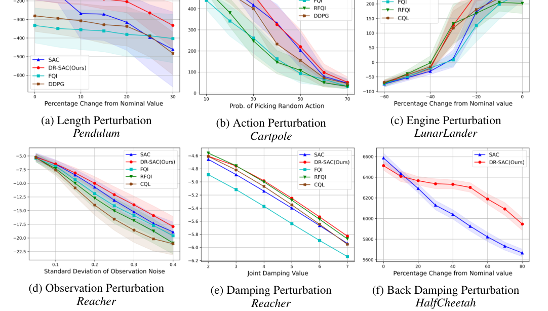
All methods are trained purely offline on transitions collected in the nominal environment (via -greedy rollouts around TD3 or SAC behavior policies, with on Pendulum, Cartpole, and LunarLander, and on Reacher and HalfCheetah) and evaluated over 50 episodes across parameter, actuator, and observation shifts. Paper, Section 4.1 and Appendix C.1, Table 3.
| Environment | Ambiguity Radius | Perturbation Axis | Headline Empirical Result |
|---|---|---|---|
LunarLander | Joint main & side engine_power; linear wind_power | At engine power shift, DR-SAC averages while SAC, CQL, FQI, and RFQI all drop below ; at engine power reduction, DR-SAC achieves the average reward of SAC. | |
Pendulum | Pole length, mass, gravity, and heavy-tailed Cauchy state noise | higher average reward than SAC at length shift; higher at mass shift; top curve across gravity shift and Cauchy noise scales. | |
Cartpole (continuous) | Random actuator probability and Gaussian observation noise | All models calibrated to nominal return; DR-SAC beats RFQI across random-action rates () and improves return by over SAC and DDPG at observation noise . | |
Reacher (MuJoCo) | Gaussian state noise (dims 4–9) and joint_damping (2.0–7.0) | Highest mean return across all observation noise and joint damping levels, with lower or comparable variance (Table 4). | |
HalfCheetah (MuJoCo) | back_damping, front_damping, and front_stiff | Under up to back_damping shift, DR-SAC holds return above while SAC falls below ; up to gain at front_stiff shift. |
Paper, Section 4.2, Figure 1, and Appendix C.2, Figures 4–6 and Table 4.
5.2 Compute accounting: functional vs. exact dual, and DR-SAC vs. RFQI
The paper’s ablation tables quantify exactly where the computational time goes on identical hardware (Ubuntu 24.04 LTS, Intel Core i7-6850K CPU with 12 cores, 64 GB RAM, and one NVIDIA GTX 1080 Ti 11 GB GPU). Paper, Section 4.3.1 and Appendices C.1 and C.3.1.
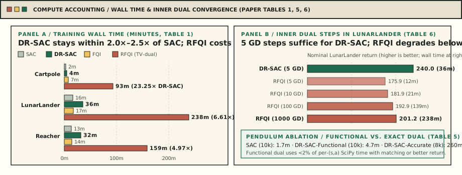
First, replacing per- scalar SciPy solves (DR-SAC-Accurate) with the shared functional network (DR-SAC-Functional, both with ) on Pendulum cuts training time by more than 98% without losing robustness:
Pendulum Variant | Training Steps | Wall Time (min) | Relative to SAC | Relative to Accurate |
|---|---|---|---|---|
SAC (non-robust baseline) | 10,000 | 1.7 | ||
DR-SAC-Functional (Algorithm 1) | 10,000 | 4.7 | ||
DR-SAC-Accurate (per- SciPy) | 8,000 | 260.0 |
Even with 25% more gradient steps, DR-SAC-Functional finishes in under 2% of DR-SAC-Accurate’s wall time, matches its return across mass perturbations up to , and outperforms it on length perturbations below . Paper, Section 4.3.1, Figure 2, and Appendix C.3.1, Table 5.
Second, across the three environments where RFQI converges, DR-SAC requires at most the training time of non-robust SAC, whereas RFQI requires 11.3–14.0× the time of FQI and up to the time of DR-SAC (saving over of training time in every case):
| Environment | SAC (min) | DR-SAC (min) | FQI (min) | RFQI (min) | RFQI / DR-SAC |
|---|---|---|---|---|---|
Cartpole | 2 | 4 | 7 | 93 | |
LunarLander | 16 | 36 | 17 | 238 | |
Reacher | 13 | 32 | 14 | 159 |
Why is RFQI an order of magnitude slower when both algorithms use a functional dual network? Table 6 of the paper isolates the reason: inner-loop conditioning. In each critic update, DR-SAC’s smooth KL log-exponential dual needs only 5 gradient descent (GD) steps on , whereas RFQI’s piecewise-linear TV dual on top of BCQ defaults to 1,000 GD steps. Truncating RFQI’s inner loop on LunarLander causes immediate degradation even in the nominal environment:
Algorithm on LunarLander | Inner GD Steps / Update | Training Time (min) | Nominal Unperturbed Return |
|---|---|---|---|
| DR-SAC | 5 | 36 | 240.0 |
| RFQI | 5 | 12 | 175.9 |
| RFQI | 10 | 21 | 181.9 |
| RFQI | 100 | 139 | 192.9 |
| RFQI (default) | 1,000 | 238 | 201.2 |
Paper, Section 4.3.1, Table 1, and Appendix C.3.1, Figure 7 and Table 6.
5.3 Generative model overhead, theoretical regret, and conservatism limits
Replacing the conditional VAE with alternative generative families confirms that sampling speed inside the Bellman backup is the governing systems constraint:
- Normalizing flows exhibit unstable training even in unperturbed
Pendulum. - Diffusion probabilistic models match the VAE’s robustness curves on
PendulumandCartpole, but iterative denoising during next-state sampling makes training at least slower than VAE-based DR-SAC. - VAE latent dimension is benign across a wide plateau: on
Pendulum(), varying produces virtually indistinguishable robustness curves (while extreme under- or over-parameterization at or degrades mildly). Paper, Section 4.3.2, Figure 3, and Appendix C.3.2, Figure 8.
On the theoretical side, Appendix D quantifies how nominal transition estimation error propagates into the learned robust policy. Suppose the estimated nominal kernel satisfies and shares support with the true nominal kernel, (Assumption D.2, which implies by Pinsker’s inequality). Then Lemma D.3 bounds the single-step operator discrepancy by
where lower-bounds the active dual temperature. Because both and are -contractions, , and the distributionally robust regret of the converged policy satisfies
Paper, Appendix D, Definition D.1, Assumption D.2, and Lemma D.3.
Both the regret bound and the KL formulation point to the two structural costs of this approach:
- Support restriction (): A KL ball only reweights transitions where the nominal model assigns positive density. A Gaussian-decoder VAE helps by smoothing empirical transitions over continuous state space, but shifts that jump outside the learned generative support cannot be anticipated by KL reweighting alone.
- Conservatism and manual radius selection (): Larger forces the critic to weight low-value next states more heavily, trading peak nominal return for a flatter degradation curve under perturbation. In the paper’s experiments, the best ambiguity radius depends on task geometry ( on
Cartpole, onPendulum, onLunarLander, and onReacherandHalfCheetah) and is chosen by grid search rather than derived automatically from local sample density. Paper, Appendix C.2.
6. Takeaways
- The bottleneck in continuous-control DR-RL is the Bellman backup, not the minimax objective. KL strong duality (Proposition 3.3) removes the infinite-dimensional transition kernel search and replaces it with an exponentially tilted expectation under the nominal model parameterized by a single scalar temperature , while preserving -contraction and monotonic soft policy improvement (Propositions 3.4–3.5, Theorem 3.6).
- Decomposable functional optimization makes the dual backup batch-friendly. By Rockafellar–Wets interchange on (Proposition 3.7), replacing per- scalar solves with a shared dual network cuts training time on
Pendulumfrom 260 minutes (DR-SAC-Accurate) to 4.7 minutes (DR-SAC-Functional)—a speedup with no loss of robustness. - Under KL duality, single-sample offline ERM silently degenerates to non-robust RL. Because is nonlinear in the transition distribution, a single offline next-state draw cancels and , forcing the optimal dual multiplier to zero. Drawing synthetic next states from a conditional transition VAE—and scoring them with an explicit SAC-v1 target value network —resolves double sampling without a simulator and runs at least faster than diffusion-based transition models.
- Smooth KL duals converge in 5 inner gradient steps where TV duals need 1,000. Across continuous-control benchmarks, DR-SAC trains in 2.0–2.5× the wall time of standard SAC and 5–23× faster than RFQI, while achieving up to higher return than SAC under severe environment perturbations.
Cite this note
@misc{zhou2026drsac,
  author = {Zhou, Duo},
  title  = {{DR-SAC: Robust to the Worst Plausible World, Cheaply}},
  year   = {2026},
  url    = {https://www.duo-zhou.com/blog/dr-sac/},
  note   = {Research note}
}